HAL 9000: (Gradient)Descent into (March)Madness Part 2: Exploratory Data Analysis

Building a March Madness Prediction Engine: Part 2 - Exploratory Data Analysis and Feature Engineering

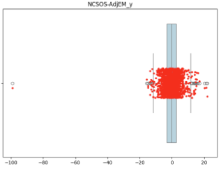
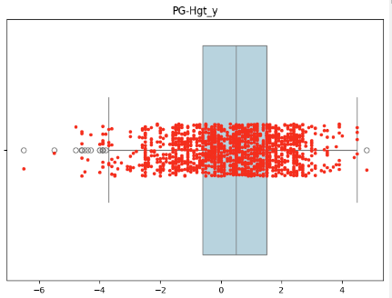
Image 1: Outlier from bad data Image 2: Natural Mugsy Bouges-Esc Outlier

With clean KenPom data acquired through the web scraping pipeline established in Part 1, the next critical phase involves understanding the statistical relationships in college basketball and engineering features that capture game-level dynamics. This process transforms individual team statistics into predictive features that distinguish between different types of basketball outcomes.

Training Data Structure and Validation

The feature engineering process begins with training datasets that combine team statistics with actual game outcomes. Three distinct datasets provide different analytical perspectives:

train_0 = pd.read_csv("../data/training_sets/train_s2010_tTrue_l0.csv")   # Tournament only
train_10 = pd.read_csv("../data/training_sets/train_s2010_tTrue_l10.csv") # + Last 10 reg season
train_20 = pd.read_csv("../data/training_sets/train_s2010_tTrue_l20.csv") # + Last 20 reg season

Each dataset contains team-pair observations where statistics for both teams (suffixed with _x and _y) are combined with three prediction targets:

• Total: Combined points scored by both teams
• Spread: Point differential (Team X score - Team Y score)
• WL: Win/Loss outcome (binary: 1 if Team X wins, 0 otherwise)

The multi-target approach enables specialized feature engineering for different prediction objectives, as total points prediction requires different statistical signals than point spread prediction.

Target Variable Correlation Analysis

Understanding which raw statistics correlate with different outcomes guides feature engineering priorities:

target_vars = ['Total', 'Spread', 'WL']
feature_cols = [col for col in train_0.columns if col not in target_vars]

# Analyze correlations with each target
for target in target_vars:
    corrs = train_0[feature_cols].corrwith(train_0[target])
    print(f"Top correlations with {target}:")
    print(corrs.abs().sort_values(ascending=False).head(10))

Total Points Correlations: Adjusted tempo (AdjT) shows the strongest correlation (0.344), confirming that faster-paced games produce higher scores. Possession-based offensive ratings also correlate strongly, indicating that efficient offenses drive scoring.

Point Spread Correlations: Net rating (NetRtg) dominates with 0.488 correlation, demonstrating that overall team efficiency differential predicts game outcomes better than any individual statistical category.

Win/Loss Correlations: Similar to spread prediction, net rating and adjusted offensive efficiency show the strongest relationships with binary outcomes.

These correlation patterns reveal that different prediction targets require fundamentally different feature engineering approaches.

Advanced Feature Engineering Framework

The sophisticated feature engineering process operates at two levels: team-level composite metrics and game-level interaction features.

Team-Level Composite Metrics

def engineer_team_features(df):
    """Create sophisticated composite metrics for each team"""
    df = df.copy()
    
    for suffix in ['_x', '_y']:
        # Ball Control - modified to avoid division issues
        df[f'Ball_Control{suffix}'] = df[f'A_Pct{suffix}'] * (100 / (df[f'NST_Pct{suffix}'] + 100))
        
        # Shot Quality - weights different shot types by value
        df[f'Shot_Quality{suffix}'] = (
            (df[f'2P_Pct{suffix}'] + 1.5*df[f'3P_Pct{suffix}'] + df[f'FT_Pct{suffix}'])/3 *
            (1 + df[f'A_Pct{suffix}']/200)  # Boost for ball movement
        )
        
        # Defensive Disruption - positive actions minus fouls
        df[f'Def_Disruption{suffix}'] = (
            df[f'Stl_Pct{suffix}'] + df[f'Blk_Pct{suffix}'] - df[f'DFTRate{suffix}']/2
        )
        
        # Free Throw Advantage - ability to draw vs allow FTs
        df[f'FT_Advantage{suffix}'] = df[f'OFTRate{suffix}'] - df[f'DFTRate{suffix}']
    
    return df

Ball Control: Combines assist rate with turnover avoidance, using a modified formula that prevents division by zero while maintaining interpretability. High values indicate teams that both create assists and avoid turnovers.

Shot Quality: Weights shooting percentages by shot value (3-pointers get 1.5x weight) and includes a bonus for assisted shots, recognizing that ball movement typically creates better scoring opportunities.

Defensive Disruption: Measures positive defensive actions (steals, blocks) while penalizing excessive fouling, capturing teams that create turnovers without putting opponents at the free throw line.

Free Throw Advantage: Differential between drawing and allowing free throws, identifying teams that attack aggressively while defending without fouling.

Game-Level Feature Engineering

The most powerful predictive features emerge from interactions between opposing teams:

def create_game_features(df, target):
    """Create target-specific game-level features"""
    df = df.copy()
    df = engineer_team_features(df)  # First create team composites
    
    if target == 'Total':
        # Features optimized for scoring prediction
        df['Pace_Factor'] = (df['AdjT_x'] + df['AdjT_y'])/2
        df['Off_Rating_Sum'] = df['AdjOE_x'] + df['AdjOE_y']
        df['Shot_Quality_Sum'] = df['Shot_Quality_x'] + df['Shot_Quality_y']
        
    else:  # Spread and WL prediction
        # Features optimized for outcome prediction
        df['NetRtg_diff'] = df['NetRtg_x'] - df['NetRtg_y']
        df['AdjOE_diff'] = df['AdjOE_x'] - df['AdjOE_y']
        df['AdjDE_diff'] = df['AdjDE_x'] - df['AdjDE_y']
        df['Ball_Control_diff'] = df['Ball_Control_x'] - df['Ball_Control_y']
        df['Shot_Quality_diff'] = df['Shot_Quality_x'] - df['Shot_Quality_y']
        df['Def_Disruption_diff'] = df['Def_Disruption_x'] - df['Def_Disruption_y']
        
    return df

This target-specific approach recognizes that total points prediction benefits from additive features (pace, combined offensive ability), while spread prediction requires comparative features (differences in team capabilities).

Comprehensive Feature Analysis

A systematic analysis reveals which engineered features provide the strongest predictive signal:

def analyze_features(train_sets):
    """Comprehensive feature analysis across all datasets"""
    for name, df in train_sets.items():
        df_features = create_all_features(df)  # Create all possible features
        
        for target in ['Total', 'Spread', 'WL']:
            # Select appropriate feature types
            if target == 'Total':
                feature_cols = [col for col in df_features.columns if '_sum' in col]
            else:
                feature_cols = [col for col in df_features.columns if '_diff' in col]
            
            # Analyze correlations and feature importance
            correlations = df_features[feature_cols].corrwith(df_features[target])
            print(f"Top correlations with {target}:")
            print(correlations.abs().sort_values(ascending=False).head(10))

Total Points Prediction Features

The analysis reveals that scoring prediction depends on pace and offensive capability:

Top Correlations with Total Points:

• AdjT_sum (Combined Tempo): 0.448 correlation
• POS_ORtg_sum (Combined Possession Offense): -0.411 correlation
• Off_Rating_Sum (Combined Offensive Efficiency): 0.410 correlation

The negative correlation with possession-based ratings reflects the mathematical relationship between pace and per-possession efficiency—slower teams often have higher per-possession ratings.

Point Spread Prediction Features

Outcome prediction focuses on team capability differentials:

Top Correlations with Point Spread:

• NetRtg_diff (Net Rating Differential): 0.642 correlation
• AdjOE_diff (Offensive Efficiency Differential): 0.573 correlation
• AdjDE_diff (Defensive Efficiency Differential): -0.542 correlation

The strong correlation with net rating differential (0.642) confirms that overall team quality gaps predict game outcomes better than any specific statistical category.

Feature Validation Through Model Importance

Ridge regression and logistic regression models validate feature importance beyond simple correlations:

# Feature importance analysis
if target == 'WL':
    model = LogisticRegression(random_state=42)
else:
    model = Ridge(random_state=42)

model.fit(X_train_scaled, y_train)
importance = pd.DataFrame({
    'feature': feature_cols,
    'importance': abs(model.coef_[0] if target == 'WL' else model.coef_)
}).sort_values('importance', ascending=False)

Model-based importance often differs from correlation analysis, revealing non-linear relationships and feature interactions that pure correlation misses.

Multi-Collinearity Detection and Management

Advanced feature engineering creates risk of highly correlated features that can destabilize models:

# Identify highly correlated feature pairs
corr_matrix = df[feature_cols].corr()
high_corr_pairs = []
for i in range(len(feature_cols)):
    for j in range(i+1, len(feature_cols)):
        if abs(corr_matrix.iloc[i,j]) > 0.7:
            high_corr_pairs.append((feature_cols[i], feature_cols[j], corr_matrix.iloc[i,j]))

# Example high correlations found:
# NetRtg_sum & AdjOE_sum: 0.822
# POS_ORtg_x & AdjT_x: -0.886

Mathematical Relationships: Some high correlations reflect mathematical relationships between KenPom metrics rather than redundant information. These require careful handling during feature selection.

Engineered Feature Overlap: Composite features sometimes capture similar underlying concepts, requiring validation that each feature contributes unique predictive value.

Feature Set Optimization

The analysis produces optimized feature sets for different modeling approaches:

Minimal Feature Sets (5-6 features)

Designed for interpretable models and rapid prototyping:

Total Points (Minimal):

minimal_total_features = [
    'AdjT_x', 'AdjT_y',           # Individual team pace
    'Pace_Factor',                 # Combined pace
    'Off_Rating_Sum',             # Combined offensive ability
    'POS_ORtg_x', 'POS_ORtg_y'   # Possession-based efficiency
]

Spread/WL (Minimal):

minimal_spread_features = [
    'NetRtg_diff',                # Overall team quality gap
    'AdjOE_diff', 'AdjDE_diff',   # Offensive and defensive gaps
    'Ball_Control_diff',          # Ball handling advantage
    'DEFG_diff'                   # Shooting defense differential
]

Medium Feature Sets (10-12 features)

Add shooting efficiency and advanced composites:

Additional Medium Features:

• Shot quality differentials
• Defensive disruption metrics
• Free throw advantage comparisons
• Strength of schedule adjustments

Full Feature Sets (15+ features)

Include all engineered features and interaction terms:

Additional Full Features:

• Style effectiveness measures
• Pace mismatch indicators
• Offensive/defensive matchup metrics
• Experience and depth factors

Feature Engineering Validation

Multiple validation approaches ensure engineered features capture meaningful basketball concepts:

Domain Knowledge Validation

Each feature maps to established basketball analytics:

• Four Factors Integration: Features incorporate shooting, turnovers, rebounding, and free throws
• Tempo Adjustment: All efficiency features account for pace differences
• Matchup Dynamics: Game-level features capture how teams interact strategically

Statistical Validation

# Test engineered features with baseline models
for target in ['Total', 'Spread', 'WL']:
    X = df[engineered_feature_cols]
    y = df[target]
    
    X_train, X_test, y_train, y_test = train_test_split(X, y, test_size=0.2, random_state=42)
    
    scaler = StandardScaler()
    X_train_scaled = scaler.fit_transform(X_train)
    X_test_scaled = scaler.transform(X_test)
    
    if target == 'WL':
        model = LogisticRegression()
        score = accuracy_score(y_test, model.predict(X_test_scaled))
    else:
        model = Ridge()
        score = r2_score(y_test, model.predict(X_test_scaled))
    
    print(f"{target} prediction R²/Accuracy: {score:.4f}")

Cross-Dataset Validation

Features validated across different training sets ensure robustness:

• Tournament-only data: Tests pure March Madness prediction
• Late-season inclusion: Validates whether regular season context improves prediction
• Temporal consistency: Ensures features remain predictive across different eras

Feature Scale and Distribution Management

Engineered features require careful scaling to ensure equal contribution to distance-based algorithms:

# Apply robust scaling to handle basketball's natural outliers
features_to_scale = [col for col in df.columns if col not in ['TeamID', 'Season']]

scaler = RobustScaler()  # More robust to outliers than StandardScaler
df_scaled = df.copy()
df_scaled[features_to_scale] = scaler.fit_transform(df[features_to_scale])

# Persist scaler for consistent preprocessing
joblib.dump(scaler, 'game_feature_scaler.pkl')

The robust scaling approach handles college basketball’s inherent outliers (extreme pace teams, unusual fouling patterns) better than standard normalization approaches.

Integration with Modeling Pipeline

The sophisticated feature engineering integrates seamlessly with the modeling framework established in the FeatureEngineer class:

class FeatureEngineer:
    def create_training_features(self, df, target_type, version='medium'):
        """Create optimized feature sets for different targets and complexities"""
        features = pd.DataFrame()
        
        if target_type.lower() == 'total':
            # Pace and scoring features
            if version in ['minimal', 'medium', 'full']:
                features['Pace_Factor'] = (df['AdjT_x'] + df['AdjT_y'])/2
                features['Off_Rating_Sum'] = df['AdjOE_x'] + df['AdjOE_y']
            
            if version in ['medium', 'full']:
                features['Shot_Quality_Sum'] = df['Shot_Quality_x'] + df['Shot_Quality_y']
                
        elif target_type.lower() in ['spread', 'wl']:
            # Differential features
            if version in ['minimal', 'medium', 'full']:
                features['NetRtg_diff'] = df['NetRtg_x'] - df['NetRtg_y']
                features['Ball_Control_diff'] = df['Ball_Control_x'] - df['Ball_Control_y']
            
            if version in ['medium', 'full']:
                features['Def_Disruption_diff'] = df['Def_Disruption_x'] - df['Def_Disruption_y']
                
        return features

This flexible architecture enables different prediction targets and model complexities to access appropriately optimized features.

Key Insights and Discoveries

The comprehensive feature engineering analysis reveals several crucial insights:

Target-Specific Optimization: Total points prediction benefits from additive features (combined pace, offensive capability), while spread prediction requires comparative features (team differentials).

Composite Feature Value: Engineered features like Ball_Control and Shot_Quality often outperform individual statistics by capturing basketball concepts that span multiple statistical categories.

Correlation Hierarchies: Net rating differential emerges as the single most predictive feature for game outcomes, validating Ken Pomeroy’s emphasis on overall efficiency.

Feature Interaction Effects: The most powerful features often result from interactions between team capabilities rather than individual team strengths.

Looking Ahead

This sophisticated feature engineering transforms raw team statistics into game-level features that capture the strategic and statistical dynamics of basketball matchups. The engineered features provide multiple entry points for different modeling approaches—from interpretable linear models using minimal feature sets to complex ensemble methods leveraging the full feature space.

The validation across multiple datasets and prediction targets ensures these features remain robust across different competitive environments and analytical objectives. This foundation enables the advanced machine learning approaches explored in Part 3, where these carefully engineered features drive predictive models capable of tournament-level accuracy.

In Part 3, we’ll explore how these features enable various machine learning algorithms to achieve remarkable prediction accuracy across different basketball outcomes.

Next: Part 3 - Machine Learning Models and Prediction Systems